Khalid Rehman1,*, Malik Altamash1, Jan Sher Khan1, Junaid Miraj1, Zaheer Farooq1
1Department of Electrical Engineering, CECOS University, Hayatabad, Peshawar.
*Correspondence: khalid@cecos.edu.pk
PJEST. 2024, 5(1);https://doi.org/10.58619/pjest.v5i1.164 (registering DOI)
Received: 19-Nov-2024 / Revised and Accepted: 21-Jan-2025 / Published On-Line: 08-Feb-2025
ABSTRACT: Load forecasting is a challenging task in the setting of modern power systems, which have risen in complexity as conventional and non-conventional energy sources have been integrated into an increasingly varied energy environment. Utility companies are under growing pressure to not just provide cost-effective and adequate power generation, but also to maintain system dependability for today’s discriminating customers. While there are several load forecasting systems, neural network-based techniques appear as a potential alternative due to their ability to reveal hidden subtleties within the input/output load data connection, resulting in fewer predicting mistakes. Artificial neural networks (ANNs)-based short-term load prediction methods have become more widely used, successfully overcoming issues related to weather, temperature, humidity, precipitation, air pressure, and the shifting patterns of human and industrial activity. This has made accurate load forecasting easier. We present FITNET, a novel feedforward neural network model designed for short-term load prediction (STLF), as our contribution to this effort. FITNET is Zunique in that it can adjust to events occurring in real time and allows training with a wide range of input kinds and sequences. We collected data from the ISO New England NE-Pool region over a period of four and a half years and combined it into a single, coherent dataset. Important inputs include time-related components and meteorological characteristics, such as day and night, dew point, and dry bulb temperature, with weekdays having a substantial impact on the output data. To improve the performance of the ANN model, we carefully examined alternate neuron configurations, using the Levenberg-Marquardt backpropagation approach for training. Extensive testing of our suggested model across both weekly and daily load forecasting methodologies continually shows outstanding efficiency, with the ANN model constantly having a forecasting MAPE of less than 1%. This finding emphasizes the model’s stability and its potential to considerably improve the dependability and cost-effectiveness of power generation in today’s complex and ever-changing energy landscape.
Keywords: ANN, FITNET, STLF, Electricity Load Forecasting, Feedforward Neural Network, Weather Parameters, Load Dataset
Introduction:
In the intricate network of our global existence, energy stands out as one of the most important resources required to support life on Earth. The growing effect of modern lives emphasizes the critical need for a consistent and adequate energy supply, which is a vital pillar of daily living [1]. Electricity is widely recognised as a cornerstone for societal growth, playing a critical role in raising the standard of living in a variety of places [2]. This global need on steady energy flow transcends geographical boundaries, serving as an essential stimulus for both developing and industrialized countries in their quest of long-term economic growth [3]. The symbiotic link between energy consumption and a country’s socioeconomic success becomes clearer, revealing a close-knit association that reflects the intertwined tapestry of global development. Unlike traditional commodities, electricity’s distinguishing feature of ‘production on demand’ emphasises its unique significance by emphasising that its distribution to end users is dependent on dynamic changes in demand [4, 5]. Addressing this requirement requires the creation of precisely constructed strategic initiatives aimed at providing an uninterrupted, secure, and adequate supply of energy, while dynamically responding to the ever-changing contours of consumer demand [6]. The strategic application of economic load dispatch is crucial in the development of power-generation systems that are not only dependable and adequate, but also economically feasible. Given the recurring and inherent fluctuations in energy demand that deviate from expected figures, load forecasting methods become inextricably linked to various aspects of power system operations, including unit commitment, stability margins, estimated available transfer capacity, load-shedding schedules, and a slew of other influential factors [7]. This complicated interaction of variables emphasises the diverse character of the energy landscape, necessitating a comprehensive and adaptive strategy to addressing the dynamic problems offered by changing consumer wants and system challenges as well.
Literature Review
As electricity businesses develop and evolve fundamentally, load forecasting technologies are becoming increasingly vital. In the 1960s, Heinemann et al. developed short-term load forecasting algorithms that were primarily focused on the temperature-load connection [8]. Following that, Lijesen et al. [9] study statistical techniques for electrical demand forecasting. Numerous approaches based on linear and nonlinear algorithms have been studied for reliable forecasting of electricity consumption. Several hybrid models that combine linear and nonlinear approaches, such as multi-layer perception and self-organizing map methods, have also aroused academics’ interest throughout the years [10, 11].
Researchers began to focus on developing non-linear approaches related to Artificial Intelligence (AI) technologies in the early 1990s [12, 13]. Data modeling flexibility was useful for ANN-based load prediction experiments. Park et al. were among the first academic groups to employ ANN in short-term load forecasting research [14]. Back Propagation (BP) Algorithm inclusion into ANN-based load forecasting was examined by researchers He et al. and Hamid et al. [15, 16]. Yang et al. devised a more precise fuzzy logic-based forecasting technique [17]. Chaturvedi et al. examined the implementation of [18].
Using New data, [19] employed deep learning. The temporal and frequency domain parameters of the model were evaluated [20].
STLF is a tactical technique that combines Artificial Neural Network (ANN) with Particle Swarm Optimisation (PSO) algorithms. According to studies [22], the foundation of this technique is a three-tiered feedforward neural network trained using the Backpropagation (BP) algorithm [23]. Notably, with a lower prediction error, the Error-Correcting Neural Network (ENN) model beats the BPNN model [23]. Another novel STLF-based time series model, described in [24], employs a K-Means clustering strategy within the ANN framework, resulting in improved prediction capabilities and much lower errors. In addition, a neural network wavelet transformation approach described in [25] is used to estimate future load levels by utilising input factors collected from comparable days’ load data.
Artificial Neural Network (ANN) Model
Artificial Neural Networks (ANNs) are mathematical algorithms inspired by organic neural systems. ANN’s basic base is an immense array of linked processing units known as neurons, with communication channels permitting data flow between these nodes. Numerous input nodes provide numerical data to the network, and the information is attenuated or amplified based on weights assigned. These weights are obtained by the use of various training patterns and adaption approaches. A neuron is activated when the synapses have the necessary weightings, and the neuron’s activity is dependent on the cumulative total of weighted inputs above a predefined threshold [21]. Figure 1 depicts the core structural model of an ANN.
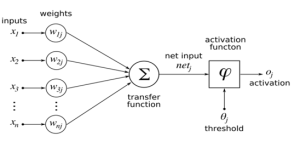
Fig. I: ANNBS (Artificial Neural Network Basic Structure)
There are three layers in a neural network. The weights between the hidden and input layers decide which neurons in the hidden unit are activated.
Leveberg – LM (Marquardt Algorithm)
Back-propagation using Levenberg-Marquardt (LM) optimum solutions is used as a network training technique to change biases and weights. The LM technique, also known as the damped least-square approach, is particularly good at tackling nonlinear least-square issues. Unlike the traditional Hessian matrix, the LM approach computes corrections using a gradient vector and a Jacobian matrix. The followingis the loss function associated with this training process:

In the first step, B = Hessian-Matrix, = Damping Factor that keeps Hessian positive, and I = Identity Matrix are chosen. If an error occurs at any iteration, the value will be increased. when loss decreases, Algorithm LM is bringing closer to the Newton approach [26].
The Mean Absolute Error (MAE) and Root Mean Squared Error (RMSE) are used to evaluate predicting effectiveness. However, the authors chose to exclude MAE and RMSE due to RMSE’s sensitivity to outliers and both measures’ scale dependency. Instead, the authors argue that Mean Absolute Percentage Error (MAPE) is a more robust evaluation measure, especially in the context of load forecasting. As a result, MAPE is chosen as the statistic for measuring the model’s expected accuracy. The MAPE formula is defined in reference [20].
Methodology
It is evaluated one output variable (actual load data) to eight input factors (daily hours. To improve the model’s efficacy, the available information was preprocessed, which included the elimination of outliers and irregular data, since ANNs are particularly sensitive to such abnormalities, negatively influencing their performance [27]
It is common practice to perform a normalization procedure before feeding inputs into the network.
We used MATLAB R2019b to train and test our suggested ANN model. Many neuron counts were investigated during the training phase, and 35 neurons yielded the best results. The output layer only has one neuron for load prediction output [27].
The learning rate is defined as the proportion of the error gradient that controls the weights. Fast convergence happens at higher levels, although oscillations become more intense. The momentum defines the proportion of earlier weight changes that are taken into account when computing new weights [27].
DATA
The authors obtained data region from January 1st, 2017 to June 30, 2021. After that, the yearly load data is put into a single data set of 39,408 data points. The data collection includes the date, hour, dry-bulb (ᵒF), dew-point (ᵒF), and system electrical load (MW).
Analysis
A key step forward in developing ANN for momentary load prediction, the necessary framework attributes should be investigated. The initial step in building any load predictor is to examine historical load records to extract load features such as periodicity and trends.
Following preprocessing, data was examined for the. The table under shows real numbers from 2017 through June 2021.
Table I: Month basis Load
| Year/Month | Jan. | Feb. | Mar. | Apr. | May | Jun. | Jul. | Aug. | Sep. | Oct. | Nov. | Dec. |
| Day/
Hour 2017 |
9/18 | 9/19 | 15/20 | 6/18 | 18/8 | 13/17 | 19/18 | 22/17 | 27/17 | 9/19 | 28/18 | 28/18 |
| 2017 Load (MW) | 19592 | 18165 | 17502 | 15843 | 20250 | 23968 | 23579 | 22769 | 20999 | 17255 | 17079 | 20524 |
| Day/
Hour 2018 |
5/18 | 7/18 | 7/19 | 3/20 | 29/18 | 18/17 | 5/18 | 29/17 | 6/16 | 10/19 | 15/18 | 18/18 |
| 2018
Load (MW) |
20662 | 18308 | 16943 | 15778 | 17518 | 21076 | 24512 | 26024 | 24475 | 17479 | 17590 | 18466 |
| Day/
Hour 2019 |
21/18 | 1/19 | 6/19 | 9/20 | 20/18 | 28/18 | 30/18 | 19/16 | 23/17 | 2/15 | 13/18 | 19/18 |
| 2019
Load (MW) |
20773 | 18585 | 17876 | 15034 | 15748 | 19913 | 24361 | 23365 | 19162 | 16138 | 17548 | 19065 |
| Day/
Hour 2020 |
20/18 | 14/19 | 1/19 | 27/18 | 29/18 | 23/18 | 27/18 | 11/18 | 10/18 | 30/19 | 18/18 | 17/18 |
| 2020
Load (MW) |
18097 | 16991 | 15888 | 14254 | 16593 | 21519 | 25121 | 24335 | 19260 | 15616 | 17157 | 18922 |
| Day/
Hour 2021 |
29/18 | 1/18 | 2/19 | 16/12 | 26/18 | 29/16 | ——— | ——– | ——– | ——– | ——– | ——– |
| 2021 Load (MW) | 18839 | 18185 | 17738 | 14649 | 18846 | 25726 | ——— | ——– | ——– | ——– | ——– | ——– |
According to the statistics, the greatest load value is 26024 MW for all the years, which happened in the seventeenth hour on 29th August 2018. Seventeenth, Eighteenth, and Nineteenth hours of the day have the highest peak load. Load increases throughout the summer months (June-September), whereas it decreases during the winter months (October-May). The MATLAB annual load graphs shown below will assist you in interpreting lines in the preceding:
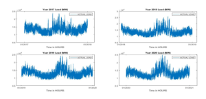
Fig. II: Yearly Actual load data
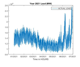
Fig. III: 2021 forecast actual load data.
In the Figure 3, demonstrates intermittent power surges and unexpected load drops throughout the year, particularly in the summer. However, overall load changes are essentially the same over time.
Data Analysis
When examining load trends over the course of a year, it is critical to account for critical factors such as weather conditions and public holidays. Previous study has shown that temperature and humidity have a significant impact on the dynamic variations in electrical load behaviour. While wind speed, air pressure, weather patterns, geographical location, public interruptions, and lock downs can all have an effect on load behaviour, they were not particularly explored in this study. Table 2 depicts the actual load fluctuations for each hour on June 30, 2021, illuminating the link with dew point and dry bulb readings.
Table II: Dew-Point, Dry-Bulb, & Actual Load Data
| Hour / Weather Information
June 30, 2021 |
Dry Bulb (ᵒF) |
Dew Point (ᵒF) |
Actual Load (MW) |
| 1 | 78 | 71 | 17,517 |
| 2 | 77 | 71 | 16,549 |
| 3 | 77 | 70 | 15,881 |
| 4 | 77 | 71 | 15,459 |
| 5 | 76 | 70 | 15,416 |
| 6 | 75 | 70 | 15,830 |
| 7 | 75 | 69 | 17,095 |
| 8 | 78 | 70 | 18,756 |
| 9 | 80 | 70 | 20,143 |
| 10 | 83 | 70 | 21,233 |
| 11 | 86 | 70 | 22,299 |
| 12 | 89 | 70 | 23,246 |
| 13 | 91 | 70 | 24,087 |
| 14 | 92 | 70 | 24,879 |
| 15 | 93 | 69 | 25,333 |
| 16 | 94 | 68 | 25,420 |
| 17 | 94 | 69 | 25,436 |
| 18 | 91 | 69 | 25,153 |
| 19 | 86 | 69 | 24,020 |
| 20 | 78 | 70 | 22,980 |
| 21 | 75 | 70 | 21,888 |
| 22 | 75 | 70 | 20,481 |
| 23 | 74 | 70 | 18,854 |
| 24 | 73 | 70 | 17,249 |
As shown in Table 2, on the load there is a little dew point effect, with the dry bulb temperature (oF) appearing as an important component trendy load variation. There is a direct association seen; as the dry bulb value increases, so does the load, and vice versa, as the dry bulb value decreases, so does the load. Figure 4 depicts graphs covering the whole dataset of dew point, dry bulb, and real load demand to present a holistic perspective, encouraging deeper examination for more insights into their interplay.
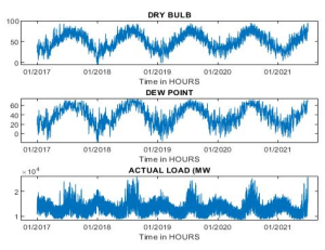
Fig. IV: Load Analysis, Dew-point, and Dry-bulb
Datasets Distribution
Datasets were divided into two broad categories: Testing Data and Training Data. In 80% of situations, data was picked for training and 20% for testing. To get the necessary weights for the ANN model, the Levenberg-Marquardt back-propagation technique was utilised. Finally, the dataset was put through its paces. After multiple trial-and-error tries with varied numbers of neurons, the precise timely network stayed chosen based on the least MAPE criteria. Hidden-layer sigmoid-transfer functions were used to evaluate the models on 20-40 neurons. 1-5 hidden layers were utilised in a trial-and-error fashion, with 35 neurons, one hidden layer, and one output layer producing the best results.
For testing purposes the month of June 2021 was picked in the second stage of the STLF forecasting procedure, then the outstanding whole previous dataset data was estimated during model exercise. During the last week of June 2021, the expected load values were tested in the third phase. The 30th of June 2021 was chosen as the last day of the fourth phase of power load forecasting. In the last stage, we forecasted the last hour of June 30th, 2021.
In this study, we concentrated on weekly and daily load data as the inputs and goal data were same throughout all stages, resulting in nearly identical outcomes.
Simulation Results
Before developing Artificial Neural Networks (ANN), a preliminary analysis was carried out with the Multiple Linear Regression (MLR) approach to determine the predicted load values for all 39,408 data points in the dataset. A comparison of the actual electrical demands (MW) and the corresponding projections produced by the MLR technique is shown in Figure 5. Notably, other inputs were not included in the study when the MLR technique was evaluated; only regular load data was taken into account.
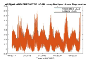
Fig. V: Predicted & actual load
When it is zoomed its results are shown more clearly as:
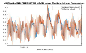
Fig.VI: Clear Plot of MLR
Findings indicates the real and expected load statistics differ significantly. Only a few deviations occur along the linear variable line, with the majority occurring under peak loads. As an outcome, the approach is ineffective for adjustable loads then effective for linearly changing loads.
In addition to applying the Levenberg-Marquardt (L-M) training procedure, the networks were also examined for Bayesian Regularisation (BR). Nevertheless, the BR approach performed noticeably worse than L-M, which resulted in its removal from the report and the conclusions drawn from it not being taken into account in the end.
Arithmetical features of the hourly, weekly, and monthly load data are shown in Figure 7, which also shows the load changes that may be observed, such as weekend decreases, month-to-month variations, and hourly variations. Since these unique load behaviour patterns are determined by network parameters, they must be examined in order to be considered when creating an appropriate Artificial Neural Network (ANN) model [28].
The results of this variation—which concentrate on the hourly load projections—are shown in the table. A detailed visual comparison of the actual load and the accompanying forecasts throughout a 24-hour period is shown in Figure 7. It is noteworthy that the trough occurred between 3 and 4 hours, while the highest load was recorded between 17 and 18 hours. This research provides insights into the temporal dynamics of load forecasts and illuminates how sensitive the model is to variations in the number of neurons.
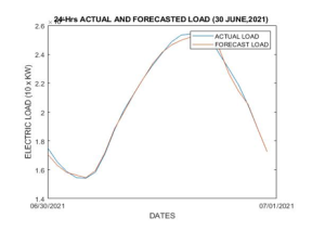
Fig. VII: 24 hours forecast & actual load
The graph showing the real and expected load shows that there are very little fluctuations throughout peak and midday hours. The graph’s stability highlights how well our Artificial Neural Network (ANN) model design predicts similar load data. The model’s aptitude for precise load forecasts is confirmed by the consistency in performance across peak and noon situations, which demonstrate the model’s resilience and dependability in capturing the underlying patterns and trends in the load data.
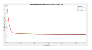
Fig. VIII: Number of EPPCH’s Against Mean Squared Error
Using the Levenberg-Marquardt back-propagation technique produced convergence after 115 iterations and 109 epochs. The results show stability post-convergence, with no appreciable increase, as seen in Figure 8. Refinement is evident in the output, which is characterised by a decrease in data loss and an increase in accuracy. There isn’t any divergence in mistakes when looking at the convergence charts for the training set.
In Figures 10 and 11, the regression plot depicting the target values against the predicted load data, and the comprehensive regression plots encompassing training, validation, testing, and overall datasets. The assessment of targeted and projected errors employs a regression measure, with Figure 12 illustrating the histogram of fit-set errors. Figure 13 provides a visual representation of both the distribution of absolute errors and the distribution of absolute percent errors, allowing for a thorough comparison of performance.
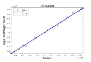
Fig. IX: Neural Network Training Curve of Performance
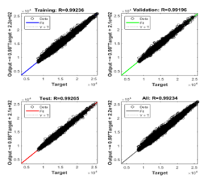
Fig. X: ANN Complete Regression Plot

Fig. XI: Histogram Error
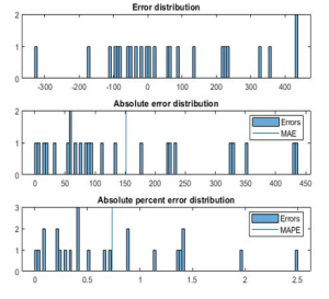
Fig. XII: Distribution Error
Table 3 depicts the projected 24-hour load data for June 30th, 2021 for each example used to estimate effectiveness by varying the number of neurons.
Table III: Actual and Predicted Loads of 24-Hours
|
Hr’s |
PL
For n = 40 |
PL
For n = 35 |
PL
For n = 30 |
PL
For n = 25 |
PL
For n = 20 |
AL
(MW) |
| 1st Hr. | 17226 | 17108 | 16853 | 17000 | 17014.5 | 17,517 |
| 2nd Hr. | 16393 | 16407 | 16054 | 16379 | 16301 | 16,549 |
| 3rd Hr. | 15970 | 15935 | 15591 | 16026 | 15892.75 | 15,881 |
| 4th Hr. | 15915 | 15764 | 15448 | 15902 | 15821 | 15,459 |
| 5th Hr. | 15772 | 15525 | 15316 | 15678 | 15573 | 15,416 |
| 6th Hr. | 16041 | 15822 | 15705 | 15950 | 15765.5 | 15,830 |
| 7th Hr. | 16883 | 16787 | 16908 | 16977 | 16780.6 | 17,095 |
| 8th Hr. | 18640 | 18730 | 18942 | 18534 | 18765.5 | 18,756 |
| 9th Hr. | 19779 | 20071 | 20108 | 19793 | 19848 | 20,143 |
| 10th Hr. | 20865 | 21182 | 21129 | 20994 | 20916.7 | 21,233 |
| 11th Hr. | 22011 | 22207 | 22108 | 22261 | 22013 | 22,299 |
| 12th Hr. | 23305 | 23328 | 23180 | 23481 | 23095 | 23,246 |
| 13th Hr. | 24468 | 24322 | 24168 | 24294 | 23938.6 | 24,087 |
| 14th Hr. | 25342 | 24964 | 24948 | 24741 | 24580 | 24,879 |
| 15th Hr. | 25986 | 25261 | 25417 | 25028 | 25113 | 25,333 |
| 16th Hr. | 26505 | 25442 | 25623 | 25365 | 25547.9 | 25,420 |
| 17th Hr. | 26808 | 25626 | 25759 | 25825 | 25871 | 25,436 |
| 18th Hr. | 26089 | 25368 | 25393 | 25460 | 25576 | 25,153 |
| 19th Hr. | 24669 | 24623 | 24579 | 24166 | 24791 | 24,020 |
| 20th Hr. | 22464 | 22837 | 22993 | 22026 | 22881 | 22,980 |
| 21st Hr. | 21121 | 21483 | 21850 | 20841 | 21465 | 21,888 |
| 22nd Hr. | 20213 | 20581 | 20893 | 20069 | 20551.8 | 20,481 |
| 23rd Hr. | 18752 | 18972 | 19280 | 18879 | 18891 | 18,854 |
| 24th Hr. | 16808 | 17104 | 17418 | 17291 | 16924.6 | 17,249 |
Table IV: Predicted Load Performance
|
|
n = 40 |
n = 35 |
n = 30 |
n = 25 |
n = 20 |
| Number of Iterations | 53 | 115 | 164 | 425 | 281 |
| Regression | 0.99222 | 0.9986 | 0.99788 | 0.99458 | 0.99510 |
| EPOCH | 47 | 109 | 158 | 419 | 274 |
| Performance | 1.1826e+05 | 1.1005e+05 | 1.1219e+05 | 1.2761e+05 | 1.1814e+05 |
In Table 4, the findings of a huge dataset including 39,385 training data points compared to a simple 24 data points during a 24-hour testing period, using hourly data received from June 30, 2021. The neural network model was rigorously tested under a variety of scenarios, each corresponding to a different number of neurons chosen, with the ultimate objective of determining the best data aggregation. When 35 neurons are used, the MAPE error is 0.73 percent, and it rises to 0.93 percent when 40 neurons are used. During the neural network training with 35 neurons, the peak performance curve reached 0.9986. As a consequence, when confronted with 24-hour test data, the best load forecasting outcomes were obtained by deploying 35 neurons within a single hidden layer, as demonstrated by the acquired findings.
The use of 30 neurons resulted in optimal weekly load analysis findings with notable accuracy. Notably, the training regression value is 0.99213, R=0.99215 summarises the total response, whereas the testing regression score is 0.99211 and the validation regression score is 0.99229. The best fit peaks at 220 epochs and 226 iterations with a strong regression value of R=0.99856, excellent performance shown by P=1.1171e+05, and a low MAPE of 1.40 percent. Figure 13 depicts the graphical display of error statistics for both weekly and hourly load data, emphasising the rigorous comparison between actual and expected loads during the final week of June 2021.
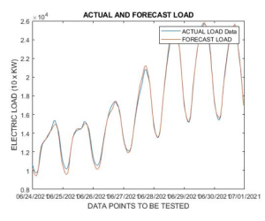
Fig. XIII: Actual and Forecast Load & Actual Data (June2021)
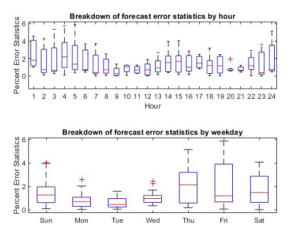
Fig. XIV: Time & Electric Load Correlation
Figure 14 highlights diverse load ranges by illustrating load distribution over various hours and days of the week. Notably, Sundays have the lowest load levels during the week, indicating a trough in the load pattern. Fridays, on the other hand, have the greatest load levels, forming the apex of the weekly load distribution. This graphic depiction captures the variations in load intensity across different days and hours, providing insights into the load profile’s dynamic character throughout the week.The expected hourly load curves follow the same pattern as the weekly load curves. There are tiny oscillations at the load peaks, and no aberrations in the load lines change linearly. To decrease these slight changes, the model will need to be fine-tuned by modifying the weights/biases and other parameters that were kept constant during our network training.
Conclusions
The method shows that ANN models may be trained using a variety of types and sequences of real-time inputs, and it was tested in MATLAB software using a Novel Feedforward (FITNET) Neural Network implementation for short-term load prediction (STLF). This data set is the result of a four-and-a-half year effort by researchers in the ISO New-England NE-Pool region. The main inputs (output data) used were time and weather variables (time, dew point, dry bulb), in addition to weekdays. The Levenberg-Marquardt backpropagation method was used to train the ANN model for various orders of neurons. We ran the model through its paces for both weekly and daily load forecast approaches to see what worked best. The network efficiency of the ANN model was improved, and it achieved two very respectable MAPE errors: 0.73% for hourly load prediction and 1.40% for weekly load forecasting.
Author’s Contribution: K. R, Conceived the idea; K. R, M. A, J. S. K, and J. M, Designed the simulated work, K. Rehman, M. Altamash, Jan Sher Khan, J. Miraj, and Z. Farooq did the acquisition of data; K. Rehman, M. Altamash, Z. Farooq, and J. Miraj, Executed the simulated work, data analysis or analysis and interpretation of data and wrote the basic draft; K. Rehman, Did the language and grammatical edits or Critical revision.
Funding: The publication of this article was funded by no one.
Conflicts of Interest: The authors declare no conflict of interest.
Acknowledgment: The authors would like to thank the advisors who advised for assistance with the collection of data.
REFERENCES
[1] M. W. Ashraf, S. Tayyaba, and N. Afzulpurkar, “Micro electromechanical systems (MEMS) based microfluidic devices for biomedical applications,” International journal of molecular sciences, vol. 12, no. 6, pp. 3648-3704, 2011. https://doi.org/10.3390/ijms12063648
[2] E. Stemme and G. Stemme, “A valveless diffuser/nozzle-based fluid pump,” Sensors and Actuators A: physical, vol. 39, no. 2, pp. 159-167, 1993. https://doi.org/10.1016/0924-4247(93)80213-Z
[3] M. J. Afzal, S. Tayyaba, M. W. Ashraf, M. K. Hossain, M. J. Uddin, and N. Afzulpurkar, “Simulation, fabrication and analysis of silver based ascending sinusoidal microchannel (ASMC) for implant of varicose veins,” Micromachines, vol. 8, no. 9, p. 278, 2017. https://doi.org/10.3390/mi8090278
[4] M. J. Afzal, M. W. Ashraf, S. Tayyaba, M. K. Hossain, and N. Afzulpurkar, “Sinusoidal Microchannel with Descending Curves for Varicose Veins Implantation,” Micromachines, vol. 9, no. 2, p. 59, 2018. https://doi.org/10.3390/mi9020059
[5] S. Tayyaba, M. W. Ashraf, Z. Ahmad, N. Wang, M. J. Afzal, and N. Afzulpurkar, “Fabrication and Analysis of Polydimethylsiloxane (PDMS) Microchannels for Biomedical Application,” Processes, vol. 9, no. 1, p. 57, 2021. https://doi.org/10.3390/pr9010057
[6] Czapaj, Rafał, Jacek Kamiński, and Maciej Sołtysik. “A Review of Auto-Regressive Methods Applications to Short-Term Demand Forecasting in Power Systems.” Energies 15, no. 18 (2022): 6729. https://doi.org/10.3390/en15186729
[7] R. Hu, S. Wen, Z. Zeng, and T. Huang, “A short-term power load forecasting model based on the generalized regression neural network with decreasing step fruit fly optimization algorithm”, Neurocomputing, vol. 221, pp. 24-31, 2017. https://doi.org/10.1016/j.neucom.2016.09.027
[8] S. Khatoon, and A.K. Singh, “Analysis and comparison of various methods available for load forecasting: An overview”, In 2014 Innovative Applications of Computational Intelligence on Power, Energy and Controls with their impact on Humanity (CIPECH), pp. 243-247, Nov. 2014. https://doi.org/10.1109/CIPECH.2014.7019112
[9] K. H. Baesmat, and A. Shiri, “A new combined method for future energy forecasting in electrical networks”, International Transactions on Electrical Energy Systems, vol. 29, no. 3, pp. 2749, 2019. https://doi.org/10.1002/etep.2749
[10] K. G. Boroojeni, M. H. Amini, S. Bahrami, S. S. Iyengar, A. I. Sarwat, and O. Karabasoglu, “A novel multi-time-scale modeling for electric power demand forecasting: From short-term to medium-term horizon”, Electric Power Systems Research, vol. 142, pp. 58-73, 2017. https://doi.org/10.1016/j.epsr.2016.08.031
[11] K. Zor, O. Timur, and A. Teke, “A state-of-the-art review of artificial intelligence techniques for short-term electric load forecasting”, In2017 6th International Youth Conference on Energy (IYCE), pp. 1-7, June 2017. https://doi.org/10.1109/IYCE.2017.8003734
[12] L. Suganthi, and A. A. Samuel, “Energy models for demand forecasting-A review”, Renewable and sustainable energy reviews, vol. 16, no. 2, pp. 1223-1240, 2012. https://doi.org/10.1016/j.rser.2011.08.014
[13] S. Ryu, J. Noh, and H. Kim, “Deep neural network-based demand-side short term load forecasting”, Energies, vol. 10, no. 1, pp. 3, 2017. https://doi.org/10.3390/en10010003
[14] K. B. Debnath, and M. Mourshed, “Forecasting methods in energy planning models”, Renewable and Sustainable Energy Reviews, vol. 88, pp. 297-325, 2018. https://doi.org/10.1016/j.rser.2018.02.002
[15] F. Rodrigues, C. Caldeira, and J. M. F. Calado, “Neural networks applied to short term load forecasting: A case study”, In Smart Energy Control Systems for Sustainable Buildings, pp. 173-197, 2017. https://doi.org/10.1007/978-3-319-52076-6_8
[16] M. Mordjaoui, S. Haddad, A. Medoued, and A. Laouafi, “Electric load forecasting by using dynamic neural network”, International journal of hydrogen energy, vol. 42, no. 28, pp. 17655-17663, 2017. https://doi.org/10.1016/j.ijhydene.2017.03.101
[17] S. Matthew, and S. Satyanarayana, “An overview of short-term load forecasting in electrical power system using fuzzy controller”, In 2016 5th International Conference on Reliability, Infocom Technologies and Optimization (Trends and Future Directions) (ICRITO), pp. 296-300, Sep. 2016. https://doi.org/10.1109/ICRITO.2016.7784969
[18] D. K. Chaturvedi, and S. A. Premdayal, “Short Term Load Forecasting (STLF) Using Generalized Neural Network (GNN) Trained with Adaptive GA”, In International Conference on Swarm, Evolutionary, and Memetic Computing, pp. 132-143,Dec.2013. https://doi.org/10.1007/978-3-319-03756-1_12
[19] Haque, S. A., & Islam, M. A. (2021). Artificial Neural Network-Based Short-Term Load Forecasting for Mymensingh Area of Bangladesh. International Journal of Electrical and Computer Engineering, 15(3), 99-103.
[20] Anand, A., & Suganthi, L. (2018). Hybrid GA-PSO optimization of artificial neural network for forecasting electricity demand. Energies, 11(4), 728. https://doi.org/10.3390/en11040728
[21] Shafiei Chafi, Z., & Afrakhte, H. (2021). Short-Term Load Forecasting Using Neural Network and Particle Swarm Optimization (PSO) Algorithm. Mathematical Problems in Engineering, 2021. https://doi.org/10.1155/2021/5598267
[22] Haque, S. A., & Islam, M. A. (2021). Artificial Neural Network-Based Short-Term Load Forecasting for Mymensingh Area of Bangladesh. International Journal of Electrical and Computer Engineering, 15(3), 99-103.
[23] Zheng, X., Ran, X., & Cai, M. (2020). Short-term load forecasting of power system based on neural network intelligent algorithm. IEEE Access. https://doi.org/10.1109/ACCESS.2020.3021064
[24] Mordjaoui, M., Haddad, S., Medoued, A., & Laouafi, A. (2017). Electric load forecasting by using dynamic neural network. International journal of hydrogen energy, 42(28), 17655-17663. https://doi.org/10.1016/j.ijhydene.2017.03.101
[25] Mohammad, S., & Hasan, M. K. An Effective Artificial Neural Network based Power Load Prediction Algorithm. International Journal of Computer Applications, 975, 8887.
[26] Nguyen, T. A., Ly, H. B., Mai, H. V. T., & Tran, V. Q. (2021). On the Training Algorithms for Artificial Neural Network in Predicting the Shear Strength of Deep Beams. Complexity, 2021. https://doi.org/10.1155/2021/5548988
[27] Rodrigues, F., Cardeira, C., & Calado, J. M. F. (2017). Neural networks applied to short term load forecasting: A case study. In Smart Energy Control Systems for Sustainable Buildings (pp. 173-197). Springer, Cham. https://doi.org/10.1007/978-3-319-52076-6_8
[28] Buitrago, J., & Asfour, S. (2017). Short-term forecasting of electric loads using nonlinear autoregressive artificial neural networks with exogenous vector inputs. Energies,10(1), 40. https://doi.org/10.3390/en10010040